After Reviewing the Waiting Line Analysis of Problem 12
Waiting Line Models
A Total Guide to Waiting Line Models and Queuing Theory
In this article, I will give a detailed overview of waiting line models. I will talk over when and how to use waiting line models from a business standpoint. In the 2d role, I volition become in-depth into multiple specific queuing theory models, that tin exist used for specific waiting lines, too as other applications of queueing theory.
Introduction to waiting line models
Waiting line models are mathematical models used to study waiting lines. Another proper noun for the domain is queuing theory.
Waiting lines tin can be set up in many means. In a theme park ride, you generally accept one line. In the supermarket, y'all have multiple cashiers with each their own waiting line. And at a fast-food eatery, you may run into situations with multiple servers and a single waiting line.
The goal of waiting line models is to draw expected result KPIs of a waiting line system, without having to implement them for empirical observation. Result KPIs for waiting lines can be for example reduction of staffing costs or improvement of guest satisfaction.
When to use waiting line models?
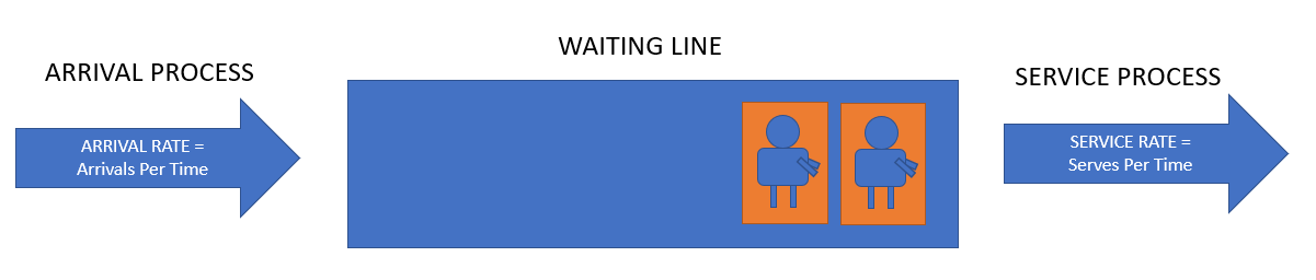
Waiting line models can exist used as long as your situation meets the thought of a waiting line. This means that there has to be a specific procedure for arriving clients (or whatever object you lot are modeling), and a specific process for the servers (usually with the divergence of clients out of the system later on having been served).
Waiting line models need arrival, waiting and service
This thought may seem very specific to waiting lines, but there are really many possible applications of waiting line models. For example, waiting line models are very important for:
- Computer processors and job handling. Many tasks arrive at the same time to your calculator'southward processor, and it has to handle them one by one without the computer failing.
- Telecommunications models. For example when many messages are being sent in a brusk fourth dimension frame and have to be dealt with correctly while limiting the "waiting time" / "delay" of the bulletin.
- Traffic engineering. For instance when many cars arrive at the same location at the same fourth dimension and they have to wait.
- Complicated multi-layer systems like call centers with multiple services are an instance of multiple waiting lines connected together.
The benefits of using waiting line models
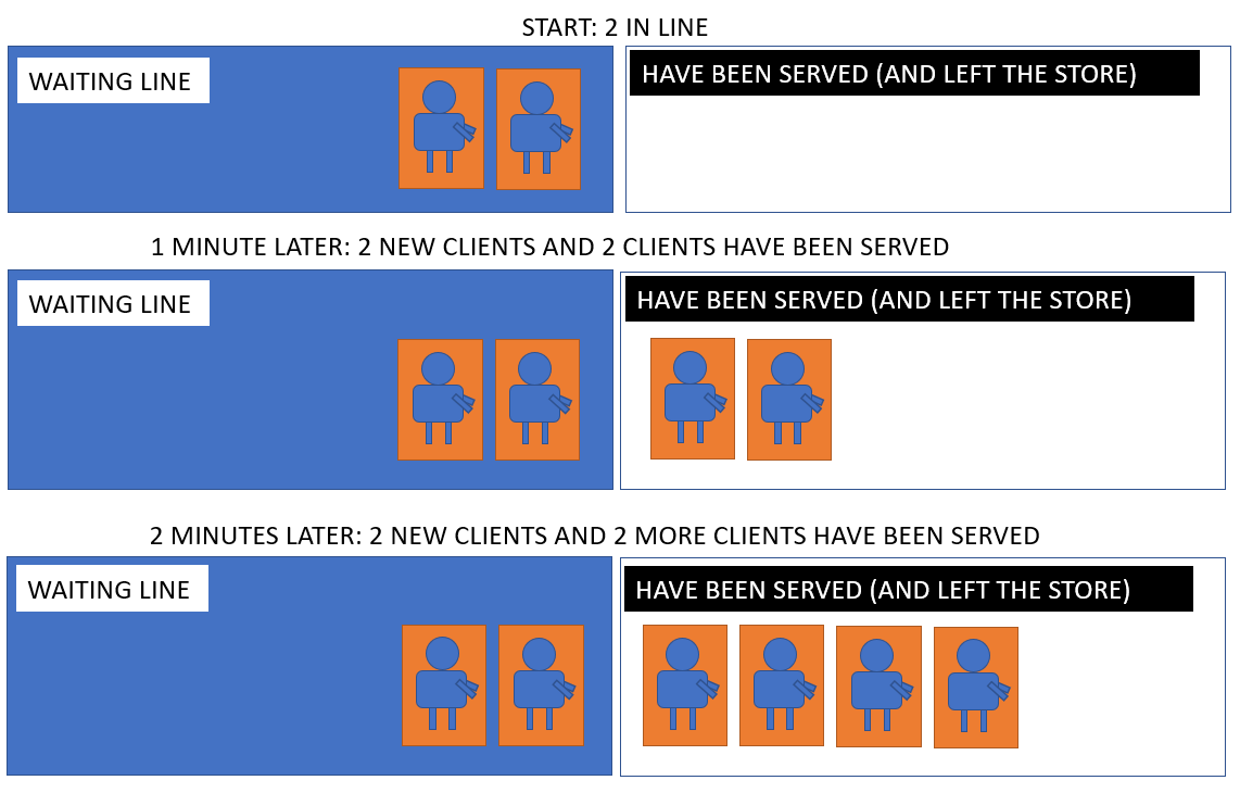
Imagine a shop with on average 2 people arriving in the waiting line every minute and two people leaving every minute equally well. That seems to be a waiting line in remainder, only then why would in that location even be a waiting line in the first place?
The respond is variation around the averages. Allow's run into an example:
Imagine a waiting line in equilibrium with 2 people arriving each minute and 2 people being served each minute:
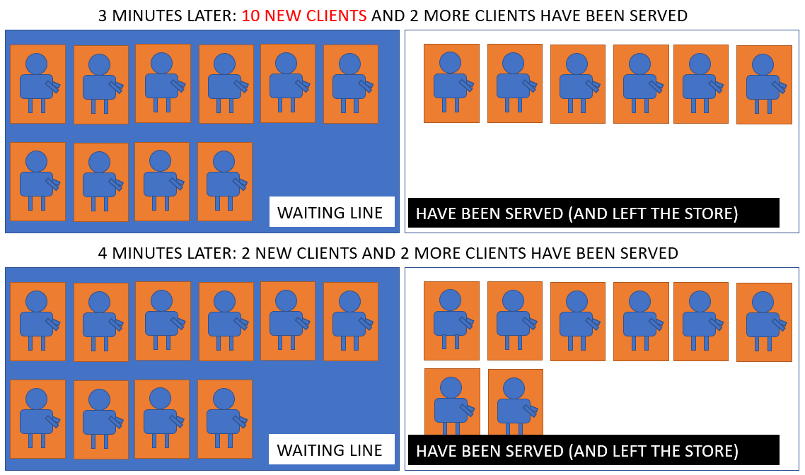
If at 1 point in time 10 people go far (without a change in service rate), there may well exist a waiting line for the residue of the twenty-four hour period:
To conclude, the benefits of using waiting line models are that they allow for estimating the probability of unlike scenarios to happen to your waiting line organization, depending on the organization of your specific waiting line.
Discover the financially optimal waiting line
An interesting business organization-oriented approach to modeling waiting lines is to analyze at what point your waiting time starts to have a negative fiscal impact on your sales.
Some interesting studies take been done on this by digital giants. For example, Amazon has found out that 100 milliseconds increase in waiting time (folio loading) costs them one% of sales (source). This type of study could be done for any specific waiting line to find a ideal waiting line organization.
Tip: discover your goal waiting line KPI earlier modeling your actual waiting line
Waiting line model KPIs
The master financial KPIs to follow on a waiting line are:
- Cost of staffing
- Cost of waiting time (opportunity cost)
- Total costs
A cracking way to objectively study those costs is to experiment with dissimilar service levels and build a graph with the amount of service (or serving staff) on the x-axis and the costs on the y-axis. This gives the following type of graph:
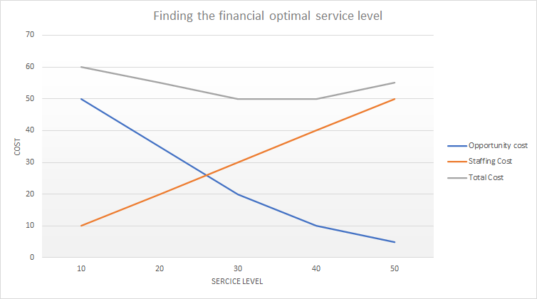
In this graph, nosotros can meet that the total cost is minimized for a service level of 30 to xl. Even though we could serve more than clients at a service level of 50, this does not counterbalance up to the toll of staffing.
Probabilistic KPIs to attain our goal-waiting line
Once we accept these price KPIs all set up, nosotros should await into probabilistic KPIs. This means: trying to identify the mathematical definition of our waiting line and use the model to compute the probability of the waiting line system reaching a certain extreme value.
Examples of such probabilistic questions are:
- What is the worst possible waiting line that would 'past probability' occur at least in one case per month?
- How many people tin can we wait to wait for more than than x minutes?
Waiting line modeling also makes it possible to simulate longer runs and extreme cases to analyze what-if scenarios for very complicated multi-level waiting line systems.
An One thousand/M/1 queue — the standard waiting line
The beginning waiting line we volition dive into is the simplest waiting line. It has 1 waiting line and 1 server.
All KPIs of this waiting line tin can be mathematically identified equally long every bit we know the probability distribution of the arrival process and the service process.
This waiting line system is chosen an M/K/1 queue if it meets the post-obit criteria:
one. Arrivals follow a Poisson distribution
The Poisson distribution is a famous probability distribution that describes the probability of a certain number of events happening in a stock-still time frame, given an average result rate.
If a prior analysis shows us that our arrivals follow a Poisson distribution (oft we volition take this as an assumption), nosotros can use the average arrival charge per unit and plug it into the Poisson distribution to obtain the probability of a certain number of arrivals in a fixed time frame.
The following case shows how likely information technology is for each number of clients arriving if the arrival rate is 1 per fourth dimension and the arrivals follow a Poisson distribution.
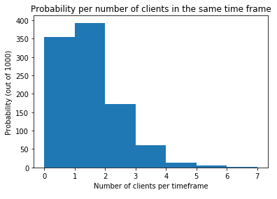
The reason that nosotros work with this Poisson distribution is merely that, in practice, the variation of arrivals on waiting lines very often follow this probability. There are alternatives, and we will see an example of this further on.
two. Service times follow an Exponential distribution
The second criterion for an Yard/1000/1 queue is that the elapsing of service has an Exponential distribution. This means that the duration of service has an average, and a variation around that average that is given past the Exponential distribution formulas.
An instance of an Exponential distribution with an average waiting time of 1 minute tin can be seen here:

Analysis of an M/One thousand/1 queue
For analysis of an M/M/1 queue we start with:
- An average arrival rate (observed or hypothesized), called λ (lambda)
- An average service time (observed or hypothesized), defined as ane / μ (mu). Service time can be converted to service rate μ by doing ane / μ.
From those inputs, using predefined formulas for the One thousand/K/1 queue, we can find the KPIs for our waiting line model:
i. Analyze the stability of our M/1000/ane queue
M/M/1 queues are stable equally long as λ < μ
Information technology is often important to know whether our waiting line is stable (meaning that it will stay more or less the same size). For the Thousand/Grand/1 queue, the stability is merely obtained every bit long as λ (lambda) stays smaller than μ (mu). This means that service is faster than arrival, which intuitively implies that people the waiting line wouldn't grow too much.
ii. Compute the utilization of our 1000/M/1 queue
A second assay to practice is the computation of the average time that the server will be occupied. This is called utilization. Utilization is called ρ (rho) and it is calculated as:
ρ = λ / μ
3. Compute the number of customers in our M/Thousand/1 queue
Information technology is possible to compute the average number of customers in the system using the following formula:
ρ / (1 − ρ)
The variation around the average number of customers is divers as followed:
ρ / ( ane − ρ)^2
4. Compute the probability of x customers being in our Thou/One thousand/1 queue
Going fifty-fifty farther on the number of customers, we can also put the question the other fashion around. Rather than request what the average number of customers is, we can ask the probability of a given number x of customers in the waiting line.
P (10 customers) = (ane − ρ) * ρ ^ x
5. Compute the average response time in our Grand/M/1 queue
The response time is the time it takes a client from arriving to leaving. It includes waiting and existence served. The boilerplate response time tin can exist computed as:
i/(μ − λ)
6. Compute the boilerplate waiting time in our M/K/1 queue
The average fourth dimension spent waiting can be computed as follows:
ρ/(μ − λ)
M/M/one queue example i
To give a practical example, permit's apply the assay on a pocket-size store's waiting line. At that place is one line and one cashier, the M/M/1 queue applies. Let'south say that the average fourth dimension for the cashier is 30 seconds and that at that place are two new customers coming in every infinitesimal.
- Stability: Arrival charge per unit λ is two customers per minute. Service fourth dimension ane / μ is 0.5 minutes, so service rate μ is 1 / 0.5= 2. We note that λ is not strictly smaller than μ so this situation is not stable.
- Conclusion: this is non a good waiting line planning, because the service is not fast enough to deal with the number of customers.
M/One thousand/ane queue instance ii
Every bit a solution, the cashier has convinced the owner to purchase him a faster cash register, and he is now able to handle a customer in xv seconds on average. Nevertheless, at some point, the owner walks into his store and sees 4 people in line. Should the owner be worried about this?
- Stability: λ is nonetheless 2 customers per minute. Service time 1/μ is 0.25 minutes, so μ is 1 / 0.25 = iv. λ is at present strictly smaller than μ then this situation is stable.
- Using formula 4. P (x customers) = (i − ρ) * ρ ^ x, we tin can compute the probability of having 4 customers waiting in line.
First, we compute ρ every bit λ / μ, which gives 2 / 4 = 0.v.
Then, nosotros compute
P ( four customers) = (1 − ρ) * ρ ^ ten
P ( 4 customers) = (1 — 0.five) * 0.5 ^ 4
P ( 4 customers) = 0.5 * 0.0625
P ( iv customers) = 0.03125 - Conclusion: the probability of having four customers in line is relatively low (around 3 out of 100). It is possible that this situation occurred with an average customer service time of 15 seconds, but unlikely. We could hypothesis that either the boilerplate customer service time may exist a bit college, or that at that place were more customers coming in at that time.
- To clinch the right operating of the store, we could try to arrange the lambda and mu to make sure our procedure is still stable with the new numbers.
Other types of queues
Now that we have discovered everything nigh the G/M/1 queue, nosotros move on to some more complicated types of queues. In order to do this, we more often than not change one of the three parameters in the proper noun. This is chosen Kendall notation.
Kendall notation
We have generally iii types of processes:
- M stands for Markovian processes: they have Poisson arrival and Exponential service time
- D stands for a fixed time between arrivals or fixed service time. D is for Deterministic.
- M stands for "any" distribution of arrivals and service time: consider it as a "non-defined distribution"
The number at the end is the number of servers from one to infinity. G/One thousand/1, the queue that was covered earlier stands for Markovian inflow / Markovian service / 1 server. Models with Yard can be interesting, but there are picayune formulas that have been identified for them. Some analyses have been washed on One thousand queues just I adopt to focus on more applied and intuitive models with combinations of Chiliad and D. Let'south have a look at 3 well known queues:
- Chiliad/Chiliad/c queue — Multiple servers on 1 Waiting Line
- M/D/c queue — Markovian arrival, Fixed service times, multiple servers
- D/M/1 queue — Fixed arrival intervals, Markovian service and one server
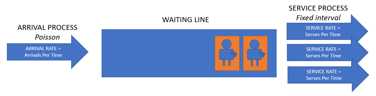
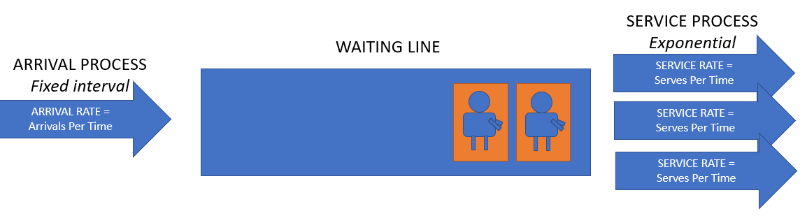
An M/1000/c queue — Multiple servers on 1 waiting line
An M/M/c queue is characterized past:
- Poisson distribution for the number of arrivals per fourth dimension frame
- Exponential distribution of service duration
- "c" servers on the same waiting line (c can range from i to infinity)
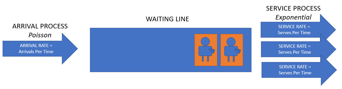
An instance of this is a waiting line in a fast-nutrient drive-through, where everyone stands in the same line, and will exist served by one of the multiple servers, equally long as arrivals are Poisson and service time is Exponentially distributed.
Its formulas are every bit follows:
- Server utilization ρ= λ / c * μ
- The queue is stable if ρ < i
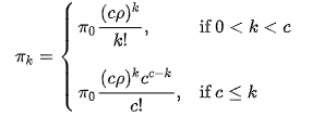
- Probability of observing ten customers in line:

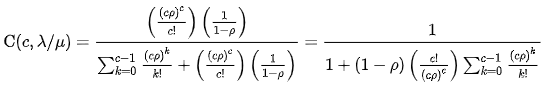
- The probability that an arriving customer has to wait in line upon arriving is:
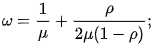
- The average number of customers in the arrangement (waiting and being served) is:

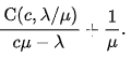
- The average time spent by a customer (waiting + beingness served) is:
An Yard/D/c queue — Stock-still service times
An One thousand/D/c queue is characterized past:
- Poisson distribution for the number of arrivals per fourth dimension frame
- Fixed service elapsing (no variation), called D for deterministic
- "c" servers on the same waiting line (c can range from 1 to infinity)
An instance of such a situation could exist an automated photo booth for security scans in airports. If nosotros accept the hypothesis that taking the pictures takes exactly the same amount of time for each passenger, and people arrive following a Poisson distribution, this would match an K/D/c queue.
In the common, simpler, instance where there is but one server, we have the Yard/D/1 example. The formulas specific for the Thousand/D/1 instance are:
- Service utilization ρ = λ / μ
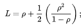
- The boilerplate number of customers in the system is
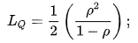
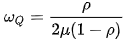
- The average number of entities waiting in the queue is computed every bit follows:
- We can also compute the average time spent by a customer (waiting + being served):
- The boilerplate waiting time can exist computed as:
- The probability of having a sure number due north of customers in the queue can be computed as follows:
When nosotros take c > ane we cannot use the higher up formulas. Nosotros need to use the following:
- Service utilization rho ρ = (λ D)/c
- The waiting line is stable as long equally ρ < 1
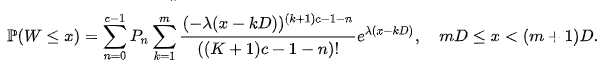
- The distribution of the waiting time is as follows:
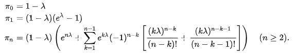
- The probability of having a number of customers in the arrangement of 'n' or less tin exist calculated every bit:
A D/G/1 queue — Fixed arrival intervals
A D/One thousand/1 queue is characterized by:
- A fixed interval betwixt arrivals (β) (D for deterministic)
- Exponential distribution of service elapsing (rate μ, mean duration one / μ) (K for Markovian)
- 1 server
The formulas specific for the D/M/1 queue are:
- The queue is stable if μβ > ane
- δ is the root of the equation δ = e ^ (-μβ(1 — δ)) with smallest absolute value.
- The mean waiting time of arriving customers is (1/μ) δ/(1 — δ)
- The average fourth dimension of the queue having 0 customers (idle fourth dimension) is β — 1/μ
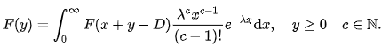
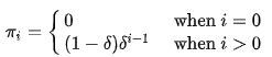
- The probability of having a sure number of customers in the system is:
Special waiting lines — overview of queue variables
In the terminal part of this commodity, I want to show that many differences come up into exercise while modeling waiting lines. In some cases, nosotros can find adapted formulas, while in other situations we may struggle to discover the appropriate model.
Here is an overview of the possible variants you could encounter
- The number of lines: some queues are split into multiple lines (either split by the system, or choice by the client)
- The number of phases: some queues are divide into multiple phases, for example in a takeaway restaurant the queue is ofttimes dissever between order and then take the food.
- Priority Rules: some queues have specific priority rules that have an effect on the throughput of the system.
- Bulk Queues: Some systems do their service in batches (eg a theme park attraction) or sometimes customers go far in batches but are served 1 by i, (eg passport control on every passenger of a plan that just landed).
- Jackson Networks: Sometimes multiple queues are interconnected at service nodes, thereby creating networks of queues. An example of a multilayer waiting line would be a call centre where you go from one agent to the other, coming closer to the exit at every footstep.
- Balking means for a client to pass up to join the queue when it is too long. This can be an important factor in a queueing system if customers are known to exist not patient.
- Reneging means leaving the queue later entering. If this happens too oft, you could think about making a two-phase queue, so that people are less likely to leave. Or meliorate the average waiting fourth dimension.
- Jockeying means switching from 1 queue to the other. This may or may non be problematic for your situation, simply it may have an event on the correctness of your computations.
Determination
After reading this article, you should have an understanding of unlike waiting line models that are well-known analytically. Cheers to the research that has been done in queuing theory, it has get relatively like shooting fish in a barrel to apply queuing theory on waiting lines in practice.
For some, complicated, variants of waiting lines, it tin can be more difficult to find the solution, as information technology may require a more than theoretical mathematical approach.
I hope this article gives you a great starting point for getting into waiting line models and queuing theory. Thanks for reading!
Source: https://towardsdatascience.com/waiting-line-models-d65ac918b26c